
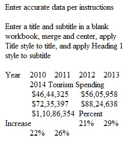
Q PC Users PC users with Office 2016 or 2013 or 365 follow directions in Excel Chapter 3 Analyzing Data with Pie Charts, Line Charts, and What-If Analysis Tools to create Project 3B. e03B_Tourism.xlsx Download e03B_Tourism.xlsx e03B_Surfers.jpg Download e03B_Surfers.jpg Project: 3B_Tourism Task Points Enter accurate data per instructions 1 Enter a title and subtitle in a blank workbook, merge and center, apply Title style to title, and apply Heading 1 style to subtitle 1 Widen column A to 150 pixels, widen B:F to 90 pixels, leave row three blank and enter row headings and column headings; apply Heading 3 cell style to column headings 1 Calculate percentage rate of increase in C6:F6, apply Accounting Number Format, decrease decimal two times, Percent style 3 Enter new title Projected Tourism Spending, copy format from A2 to A8; enter text under title, Bold and Italic; enter row and column titles, apply Heading 3 style 1 Calculate percentage rates of increase with 25% and 21% increases over five years and paste the values, not the formulas 2 Create title for estimated growth, enter row titles, copy format from A8 to A15; apply Fill Color, Theme White, Background 1, Darker 15% to A10:B10 1 Change Theme colors to Orange 1 Create a line chart with markers using Tourism Spending figures; Reposition upper left corner of chart to cell A8; Create Chart Title, format title Bold, font Black, Text 1 2 Edit category axis to use years as category names 2 Adjust axis in line chart to show minimum value of 4,000,000 and value increase in increments of 2,000,000 2 Insert picture e03B_Surfers as fill in chart, add a solid line picture border, width 4 pt, rounded corners 1 Format Vertical and Horizontal Axis with Bold and Black, Text 1 font; Plot Area gridlines set to 1 pt, orange 1 Insert footer with file name, add document properties with name and keywords; Page Setup Center Horizontally 1 Total Points 20 Copyright © 2014 Pearson Education, Inc. Publishing as Prentice Hall Mac Users Mac users with Office 2016 or 2011 or 365 follow directions in Excel Chapter 3 Analyzing Data with Pie Charts, Line Charts, and What-If Analysis Tools to create Project 3B. e03B_Population_Growth.xlsx Download e03B_Population_Growth.xlsx e03B_Beach.JPG Download e03B_Beach.JPG Project: 3B_Population_Growth Task Points Enter accurate data and format per instructions 2 Calculate and format percentage rate of increase in C7:F7 2 In B31:F31, calculate percentage rates of increase for three rates and paste the values, not the formulas, in B36:F38 6 Create a line chart using A6:F6 population figures, remove legend, change chart title 2 Adjust axes in line chart to show minimum value of 100,000 and increments of 10,000 2 Insert picture in chart area, plot area set to none, border and rounded corners applied, gridline and label color changed 2 Edit category axis to use years as category names 2 Remove unused worksheets 1 Insert footer with file name, add document properties with name and keywords, page layout in Portrait and centered horizontally 1 Total Points 20 Copyright © 2013 Pearson Education, Inc. Publishing as Prentice Hall PreviousNext
View Related Questions